
To Gamble or Not to Gamble in Kaggle's March Madness Competition
Kaggle is running their annual March Madness competition (third year). This is my first year participating. The competition asks you to predict the games of the NCAA tournament (all 68*67/2=2278 possible match-ups) by submitting probabilities that one team will win. You are judged based on the (negative) average log-losses of your predictions.
Log-loss is the natural logarithm of 1 minus your "miss". If you predict a team has a .1 chance of winning, and they lose, your miss for that game is .1. 1 minus your miss is .9. Your log loss for this game is -log(.9)=.105.
Here is a plot of Log-loss versus miss for one prediction/game:

You are judged by the average of your log-losses through all the observed 63 games (the play-in games don't count).
There are many competitors in this competition. Each competitor can submit up to two different sets of predictions. This makes for roughly 1500 different entries all trying to predict the same tournament.
Each competitor (me included) is making a model to predict the games based on historical results. The prizes are as follows: $10,000 for first place, $6,000 for second, $4,000 for third, $2,000 for fourth, and $1,000 for fifth.
A popular topic talked about is whether there is an incentive to extremize your predictions or employ some other scheme in order to differentiate yourself from the pack of competitors and have a better chance of winning.
If your goal is simply to make the best prediction you can, and thus be as high as you can be on the leaderboard on average, you should go with the predictions that your model spits out. Assuming you've done the training and testing correctly, the model is doing the best it can do to minimize that score.
Interestingly though, if your goal is only for the money earned by placing within the top 5, the optimal strategy changes. Since everyone is competing for those five places, making predictions that are close to the mean predictions of the pack actually hurts your chances of placing within the top 5, even if those predictions are the true odds associated with each game.
This is why I like the choice of the contest administrators to allow two different submissions by each competitor. The competitor doesn't have to choose one goal or the other but instead can target one goal with each submission.
I employed simulation to try to help answer the question of what the optimal strategy is for the second goal of having the most expected earnings.
It first simulates the "true odds" for each of the 63 games of a tournaments from a beta distribution. I used the parameters alpha=.65, beta=.65 so the distribution is heavy tailed. This decision was informed by simulating tournaments and looking at the average log-loss scores for predictions that were exactly the true odds. If the parameters are above one, the games are too hard to predict. As the parameters get smaller, the games become easier to predict. I looked at past contest winners' scores to help make this decision. Admittedly, this is not the most informed decision since there have only been two years of competition, but I don't think this should impact the results too much.
First let's start with the simple scenario that somehow every competitor knows the "true odds" associated with each game.
Let's look at the extremizing strategy. Here's the extremizing function:
It takes in two parameters: a vector of predictions (one for each of the 63 games) and a tuning parameter that indicates what percent to extremize by. For example, a game with a prediction of .6 and a tuning parameter of .5 will come out as (1-.6)*.5+.6 = .8.
In order to guard against predictions of 0 or 1 when competitors employ extremizing with a = 1 , I will use this simple "cap" function:
Let's say that some of the competitors decide to employ this strategy of extremizing. To evaluate the merit of this strategy, I made 900 virtual competitors. As the index of the competitor increases, the more the competitor extremized his or her predictions. Here is the structure of the simulation:


Log-loss is the natural logarithm of 1 minus your "miss". If you predict a team has a .1 chance of winning, and they lose, your miss for that game is .1. 1 minus your miss is .9. Your log loss for this game is -log(.9)=.105.
Here is a plot of Log-loss versus miss for one prediction/game:

You are judged by the average of your log-losses through all the observed 63 games (the play-in games don't count).
There are many competitors in this competition. Each competitor can submit up to two different sets of predictions. This makes for roughly 1500 different entries all trying to predict the same tournament.
Each competitor (me included) is making a model to predict the games based on historical results. The prizes are as follows: $10,000 for first place, $6,000 for second, $4,000 for third, $2,000 for fourth, and $1,000 for fifth.
A popular topic talked about is whether there is an incentive to extremize your predictions or employ some other scheme in order to differentiate yourself from the pack of competitors and have a better chance of winning.
If your goal is simply to make the best prediction you can, and thus be as high as you can be on the leaderboard on average, you should go with the predictions that your model spits out. Assuming you've done the training and testing correctly, the model is doing the best it can do to minimize that score.
Interestingly though, if your goal is only for the money earned by placing within the top 5, the optimal strategy changes. Since everyone is competing for those five places, making predictions that are close to the mean predictions of the pack actually hurts your chances of placing within the top 5, even if those predictions are the true odds associated with each game.
This is why I like the choice of the contest administrators to allow two different submissions by each competitor. The competitor doesn't have to choose one goal or the other but instead can target one goal with each submission.
I employed simulation to try to help answer the question of what the optimal strategy is for the second goal of having the most expected earnings.
It first simulates the "true odds" for each of the 63 games of a tournaments from a beta distribution. I used the parameters alpha=.65, beta=.65 so the distribution is heavy tailed. This decision was informed by simulating tournaments and looking at the average log-loss scores for predictions that were exactly the true odds. If the parameters are above one, the games are too hard to predict. As the parameters get smaller, the games become easier to predict. I looked at past contest winners' scores to help make this decision. Admittedly, this is not the most informed decision since there have only been two years of competition, but I don't think this should impact the results too much.
trueprobs<-rbeta(63,.65,.65) ##true probabilities of the games
First let's start with the simple scenario that somehow every competitor knows the "true odds" associated with each game.
Let's look at the extremizing strategy. Here's the extremizing function:
extremize<-function(x,a){
x[x>.5]<- x[x>.5]+(1-x[x>.5])*a
x[x<.5]<- x[x<.5]-x[x<.5]*a
return(x)
}It takes in two parameters: a vector of predictions (one for each of the 63 games) and a tuning parameter that indicates what percent to extremize by. For example, a game with a prediction of .6 and a tuning parameter of .5 will come out as (1-.6)*.5+.6 = .8.
In order to guard against predictions of 0 or 1 when competitors employ extremizing with a = 1 , I will use this simple "cap" function:
cap<-function(x){
x[x<=0]<-.001
x[x>=1]<-.999
return(x)
}
Let's say that some of the competitors decide to employ this strategy of extremizing. To evaluate the merit of this strategy, I made 900 virtual competitors. As the index of the competitor increases, the more the competitor extremized his or her predictions. Here is the structure of the simulation:
for (s in 1:numofsims){
scores<-numeric(numofcomp) ##vector for scores
outcomes<-rbinom(63,1,trueprobs) ##draw to simulate game outcomes
for (i in 1:numofcomp){
assessments[,i]<-cap(extremize(trueprobs,(i-1)/900))
#the bigger the index of the competitor, the more he or she extremized
scores[i]<-logloss(assessments[,i],outcomes)
}
score<-sort(scores,index.return=TRUE)$ix
placement<-placement+rank(scores)
money[score[1]]<-money[score[1]]+10000
money[score[2]]<-money[score[2]]+6000
money[score[3]]<-money[score[3]]+4000
money[score[4]]<-money[score[4]]+3000
money[score[5]]<-money[score[5]]+2000
##record the competitors who earned money and the finishing order
}
Now for the results of this strategy. To get an idea of what the competitors predictions were like, let's look at the predictions for one specific game. Game 4 has "true prob" = .55. Here are the competitors predictions for this game:
 So the competitors with the higher id are taking more risk - "gambling".

Let's see how the competitors faired in terms of average placement on the leaderboard through all the simulations (I did 700).
 Interestingly, the competitors that extremized a little bit did the best in the average leaderboard position. As of now, I really don't know why this is the case. It runs counter to the hypothesis that the best strategy for leaderboard placement is just submitting the "true odds". This has nothing to do with some sort of glitch in the rankings having to do with ties since there are never ties. Anyway, this is not really a pronounced affect but it is interesting. Onwards.
Now for the money! Let's see how the competitors faced in average money won.
 Yikes, that is ugly. Seems like practically no one except the first couple competitors won any money. Let's take a look at log(money) to get a clearer picture.


Now for the money! Let's see how the competitors faced in average money won.


There is a sharp drop off from competitor 4 to competitor 5. In fact there is a fairly perfect monotonically negative relationship between money won and amount extremized. Here are the first six values in the average money won vector:
5057.14286 3050.00000 2057.14286 1580.00000 1051.42857 31.42857
Ok. Some clarity, some more questions. Let's move on and look at another strategy. Sticking with the basic assumption that everyone knows the true odds associated with each game, let's have competitors add random amounts of noise to their predictions with the hopes of distinguishing themselves from the crowd.
Here is a function I call perturb (name inspired by this thread in the Kaggle competition):
perturb<-function(x,a){
return(x+rnorm(length(x),0,a))
}
"perturb" takes in two inputs: a vector of predictions, and a tuning parameter for how much noise to add.
Now, instead of each competitor extremizing by an amount proportional to his or her index number, the competitors will add an amount of noise proportional to his or her index number.
assessments[,i]<-cap(perturb(trueprobs,(i-1)/2500))
I choose the 2500 because they seemed like nice amount to start with. We can try different amounts of noise later. So the competitors with low indexes will have predictions that are perturbed very small random amounts, and the competitors at the end will have predictions that are perturbed by much larger amounts. Competitor #1 will not have noise added to his or her predictions. Competitor #900 will have noise with N(0,.36) added to all of his or her predictions..
Now let's first by looking at the predictions of the competitors for a single game to get a sense of what's going on. Game #8 in this simulation had "trueprob" .67. Here are the predictions of the competitors for this game:
 So yes, this seems to be a lot of randomness to add. Some of the predictions of the competitors with higher id's are around 0.
Let's see the average leaderboard positions of the competitors:
 As expected, the average finish of the competitors with the most accurate predictions (least amount of noise added) is the best. It is a monotone relationship.
Now, what about the average money won? Drumroll please....
Now let's first by looking at the predictions of the competitors for a single game to get a sense of what's going on. Game #8 in this simulation had "trueprob" .67. Here are the predictions of the competitors for this game:

Let's see the average leaderboard positions of the competitors:

Now, what about the average money won? Drumroll please....

So, perhaps surprisingly, the peak of average money won occurs not for those competitors who had the most accurate predictions, but instead for the competitors who added noise. Most surprising to me is the fact that none of the first 88 competitors made ANY money. The accuracy of their predictions lost to the randomness of the rest of the field's predictions for placement inside the top 5. Even the competitors who added lots of noise beat those with the most accurate predictions.
Ok, so this is perhaps interesting. But is it a by product of the simple assumption made that everyone knows the "true probability" associated with each game?
Let's test this out by adding a wrinkle. Let's say now, there are different classes of accuracy. Let's say 30 classes. 1 group know the correct odds perfectly (they spent a lot of time on their model or they're just really smart). The next group is a little less accurate, and so on and so forth until the last class is not very accurate at all.
Here's a function for making prediction inaccurate:
make_inaccurate<-function(x,a){
return(a*runif(length(x))+(1-a)*x)
}
x is again the vector of predictions, a is again a tuning parameter. This time a indicates what percent of a random uniform variable to use as the prediction. If a is 0, the predictions are returned as is. If a is 1 the predictions are changed to random predictions.
Now the first 30 of the 900 competitors are the smart ones so they're predictions will be the trueprobs. The last 30 of the 900 will have completely random predictions.
The goal is to test the two strategies - extremizing and adding noise - to see how they fare intragroup. Is there a benefit to employing either of these strategies to gain an advantage towards one of the goals against the competitors in your class of accuracy? Is the benefit/detriment different between the classes? Let's see.
The trueprobs will now be replaced with fakeprobs:
fakeprobs<-matrix(0,63,numofclasses)
for (i in 1:numofclasses){
fakeprobs[,i]<-make_inaccurate(trueprobs,(i-1)/100)
}
Each classes' size is 30. 100 is again a random choice. It makes it so the final class will have 30 percent random guesses along with 70 percent of the trueprobs for their predictions. Here is a plot of the amount of random guess incorporated in assessment for all the competitors:

Now, let's test the strategies intragroup. First the extremizing strategy:
assessments[,i]<-cap(extremeize(fakeprobs[,(i-1)%/%numofclasses+1],(i-1)%%numofclasses/(numofclasses-1)))
Class members with the lowest index number will not extremize and class members with the highest index number will extremize as much as possible.
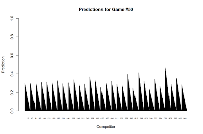
First let's start by looking at what the predictions look like for a particular game. In this run, the true probability of game #50 was .30. Here are what the predictions look like for all the competitors now:

As you go to the right the predictions of a particular group are less accurate, and as you go to the right inside a particular group, the predictions are more extremized. For games with trueprobs close to .5, the picture will look a little bit strange since some of the groups might come to the conclusion that the odds are on the wrong side of .5 and so will extremize in the exact wrong direct. But such is the risk of extremizing.
Let's take a look at the results intragroup across all simulations of average placement on the leaderboard. Let's start with group 1:

This result is the same as it was the first time around and is the same globally this time around as well as within each group: it does not make sense to extremize for the sake of placement on the leaderboard.
Now what about extremizing for the sake of average money won within a group? Let's start with group 1:

That's a bit different. The competitor who earned the most extremized the least as before, but now the competitor who extremized the most actually came in second place. Is this just random noise? Possibly. This is only the result of 700 simulations. Let's take a look at another group..

Wow, this is a large difference. Perhaps it does pay to extremize for the sake of winning money, especially for those with less accurate models. Let's take a look at another group. Say #7:

More simulations must be run to come to a more confident conclusion. Initially, it seems that it might pay to employ extremizing for those with less than the best models.
Ok, finally, what about the second strategy of adding random noise to predictions. When every competitor had the same baseline accuracy, the results were that there was no point in terms of leadership placement to add noise. However, towards the goal of money earned, there was a benefit of adding random noise. Will the same hold within accuracy classes? Will there be a difference in this effect between different groups?
First, the code for this strategy:
assessments[,i]<-cap(perturb(fakeprobs[,(i-1)%/%numofclasses+1],(i-1)%%30/81))
I chose 81 specifically because it is about the same amount of noise that (i-1)/2500 yielded at the extreme indexes when all the competitors were in one large accuracy class.
First, here are the predictions for one game and one group. Here's Group 1's prediction for game 5. Game 5 trueprob was .46:
 Ok, how did adding random noise affect average leaderboard placement within an accuracy class? I will spoil the surprise, and for the sake of brevity, tell you that it was the same as with one big accuracy class, it was uniformly bad for average leaderboard placement to add random noise no matter what accuracy class you were in.
But what about Money within an accuracy class? Did it help for average money earned to add random noise just as it did before? Let's take a look. Group #1:

First, here are the predictions for one game and one group. Here's Group 1's prediction for game 5. Game 5 trueprob was .46:

But what about Money within an accuracy class? Did it help for average money earned to add random noise just as it did before? Let's take a look. Group #1:

This pattern looks very similar as before! No money won by the competitors who did not add any noise. The peak is somewhere around 1/3 of the way to the extreme (note this will probably depends on the amount of noise added relative to index number which I have just chosen arbitrarily).
Let's take a look at just one more group to see if the pattern is similar.

Let's take a look at just one more group to see if the pattern is similar.

Again, similar pattern.
Conclusion
I don't think anything new was really discovered towards the goal of average placement on the leaderboard but certainly interesting results as to the strategy one should employ towards the goal of winning the most money on average.
There is definitely more that can be done here.
Thinking about how much noise precisely to add to your predictions to most positively impact your average money won is one question. Also, should your decision depend on what you think others will do?
Also, which is better extremizing or adding noise and for who (i.e. what accuracy class). I did not really compare the two strategies directly but instead analyzed each separately.
I'd welcome feedback!
Here is the R code for this project.
Written on March 5, 2016