Introduction and Motivation:

I seek to answer the question of what is the probability of a candidate winning an election (or caucus) when not all the votes are in. Now I will not take in any other information than votes collected for each candidate and percent of votes collected so far.

I will talk about my first approach and then talk about where I went from there and then finally what someone who really knows what they are doing might do when trying to answer this question.

For anyone who was watching the Iowa Caucus on February 1, 2016 (to which the title refers to), you probably know that some of the most crucial information to answering the question of does Bernie have a chance is what percent of the votes have been reported from all the different counties. On CNN, they would show an overall percent of precincts that have reported but they'd also show the percent that have reported from all the different counties - some of which might be more pro-Bernie than average or more pro-Hillary than average, etc. One of the most fun parts of watching the debate was speculating what the chances are at any given moment of each candidate winning. From this experience and wanting to practice and develop my stat-comp skills, I became interested in working on this problem. 

The programs that I wrote treat the whole state as one giant population. If you had realtime access to the information that CNN has, you could extend this technique to incorporate a sum of all the different counties, treating each one as a separate population of voters. This would certainly add accuracy. For now, to keep things simple, I will treat the whole state as the same population. Also, I will ignore the fact that in the Democratic Caucus, each candidate is awarded delegates according to how well they do at each voting site. Because I don't know the rules that govern this process, I'll ignore this fact. So yes, this is a theoretical exercise..

I will make the assumption that the votes will be counted randomly from a basket of votes. This seems reasonable - the votes will be thrown in a basket all together and be plucked out randomly.

First Approach:

There are two sources of uncertainty in the problem. One is estimating the true proportion of the population of voters that plan to vote for each candidate. I've always been taught to approximate the distribution of this proportion using the normal distribution. If we say the true proportion of voters who plan to vote for a candidate is , the number of votes for a candidate is , and the total votes is , then, . I use for Gaussian distribution so as not to get confused with , the total number of votes seen so far.

The next source of uncertainty in the problem is in estimating the number of total votes each candidate will eventually get. Given some population proportion of voters who plan on voting for a candidate, this source of uncertainty translates to not knowing who actually showed up on voting day. If we say  is the number of votes a candidate will eventually get, and  is the number of votes yet to be seen, then given , can also be approximated by a normal random variable:

.

Now the trouble is the Xs are not independent of one another. In other words, the candidates are competing for votes. The Xs actually belong to a multinomial distribution. Given and , . The number of votes for each candidate has a negative correlation.

My first approach was to do a simulation. With each simulated election there were different population proportions generated from random draws from normal distributions. This was my approach to an election between two candidates with some made up numbers (in pseudo-code - it's like half R, half Python):

n1=350 ##votes for cand. 1
n2=400 ##votes for cand. 2
N=sum(n1,n2) ##total votes
prctObs=.15 ##percent of votes observed thus far
V=N/prctObs-N ##number of votes yet to be counted
numOfSims=100000 ##number of simulations
votesfor1=numeric() ##empty vector to hold number of votes for cand. 1
votesfor2=numeric() ##empty vector to hold number of votes for cand. 2
for i in 1:numOfSims
    phat1=rnorm(n1/N,sqrt(1/N*n1/N*(1-n1/N))) ##1 random normal pop. proportion
    phat2=rnorm(n2/N,sqrt(1/N*n2/N*(1-n2/N))) ##another random normal pop. proportion
    phat1=phat1/(phat1+phat2) ##standardization (so probabilities will add to one)
    phat2=phat2/(phat1+phat2) ##standardization
    m=rmultinorm(V,c(phat1,phat2)) ##simulating the rest of the votes from a multinomial distribution
    votesfor1.append(n1+m[1]) ##record number of votes for cand. 1 in this election
    votesfor2.append(n2+m[2]) ##record number of votes for cand. 2 in this election

If you were very astute in checking that code out, you'll notice that I made an important choice that I have not yet discussed. Within each election, I standardized the population proportions so that the sum will add to 1. I did this because it feels right - they are probabilities, they should add to one. Also the properties of this process seem to mirror the real life situation. If, according to random chance, we are underestimating one candidates population proportion, that means we should be taking away from the other candidates' proportions. This means that random variables that are the population proportions are negatively correlated as well.

The simulation runs fairly quickly - 100,000 election simulations takes roughly 5 seconds. To get the probability of each candidate winning, all one must do is keep track of the number of times each candidate came out on top and divide by the total number of simulations.

Here are some sample elections. I divided 150,000 votes up - 46.4% for Sanders, 46.8% for Clinton and then rest for O'malley:

Votes for Hilary Clinton - 74850          Votes for Bernie Sanders - 74400          Votes for Martin O'malley - 900
Percent of Votes Observed  - 90%

Probability of each candidate winning: Clinton - .99991, Sanders - .00009, O'malley - 0.

So, under the naive assumption that the whole state is one population and that the votes are coming in randomly, even through Clinton is only 450 votes ahead with about 16,666 votes yet to be counted, she is virtually assured of victory. Let's say the same proportion of votes have come in but this time on 80,000 votes observed and 50% of the expected number of votes.

Hilary Clinton - 39840           Bernie Sanders - 39680          Martin O'malley - 480
Percent of Votes Observed  - 50%

Probability of each candidate winning: Clinton - .822, Sanders - .178, O'malley - 0.

The results seemed strange to me. Of course these numbers do not currently properly model the real life scenerio on account of the fact - as I mentioned - that I am treating the entire state as one population. Still the simulation seemed to be overly bullish for the favorite. Here are some more runs of the simulation with some hypothetical scenarios. Maybe you'll agree with me, maybe you won't.

Votes for Candidate 1 - 134          Votes for Candidate 2 - 130
Percent of Votes Observed - 2%

Probability of each candidate winning: Candidate 1 - .64, Candidate 2 - .36.

Votes for Candidate 1 - 134          Votes for Candidate 2 - 130
Percent of Votes Observed - 76%

Probability of each candidate winning: Candidate 1 - .70, Candidate 2 - .30.

Perhaps the numbers are where they "should be". Still, I was unsatisfied and wanted a way of calculating the real distributions that the determine the probabilities.  I didn't want to rely solely on simulations. So I tried my best to do it.

My next approach:

Regrettably, I took sort of a parochial approach to trying to solve for the real probabilities. Based on how I was going about the simulation, I tried to calculate the explicit probabilities using the same model. It did not really occur to me that if I did succeed, the numbers would come out exactly the same.  -_-

Nonetheless, it was good practice.

I started by asking what kind of distribution

should have where are independent Gaussians. Well, unfortunately this whole distribution sort of fails on account of the denominator being potentially equal to 0. One could try to limit X,Y, and Z to the domain (0,1] and divide each pdf by
 and then perform the triple integral to get the mean and variance of this cockamamy distribution. Instead of doing that, I just simulated these quantities. The great thing about random number generation is that the chances of the sum of these three random variables being exactly 0 is basically 0. Especially considering the the sum of the expectations of the random variables in the denominator for this problem will always be 1.

I set up the problem like this:




I calculated all the v's and c's from simulation. In general all the v's were fairly similar to the variances of the normal distributions sampled from. All the c's were negative - except those on the diagonal of course - which makes intuitive sense since the higher one population proportion is, the lower any other is.

Then, from these formulas I calculated the first two moments of the X's and the covariance between them:


                  

                         
Each component of the covariance is negative since each c is always dominated by the (n/N)*(n/N) term. I am not quite sure why Cov(Xi,Xi) ≠ Var(Xi). There is an additional V*(ni/N) positive term in the variance formula that makes both components of it positive. I confirmed these formulas with simulations.

Also with simulations, I confirmed that the distributions of the Xs look pretty normal.

So now the problem boils down to trying to find:  since that is that probability of candidate 1 winning and then to calculate that for each of the k candidates.

Luckily, smart people have been working on this problem, especially for the case of the max of a series of Gaussians. The normal strategy for this problem seems to take the pairwise max of each of the random variables in the series- taking advantage of the fact that. For Gaussians the pdf(t) of max(X,Y) with correlation coefficient  looks like this:

Bayesian Approach:

The two (really one) approaches I have taken so far are both frequentist approaches. There is another way of approaching the problem that many people would choose - the Bayesian Approach. This requires setting a prior distribution for the population proportions of the candidates. If one were really doing this seriously, experimenting with different prior distributions would be crucial to fine tuning the calculation.

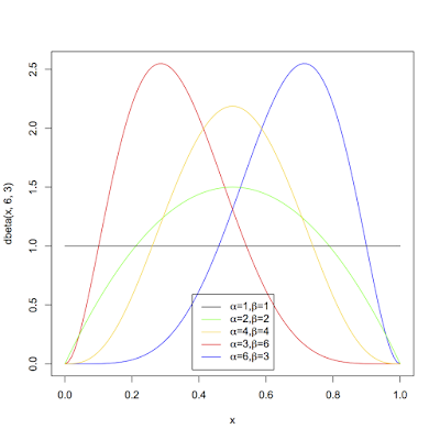
First, I will compute the probability for two candidates. This, should be simple. There is a nice solution with the Beta-Binomial distribution. Since there are only two candidates to vote for, each vote is like a coin flip heads or tails. The prior distribution is a Beta distribution. Depending on the parameters chosen, the distribution can look wildly different:
Polling would be an obvious way to choose a prior distribution. I'll make two computations, one with a naive prior - alpha = 1, beta = 1 - and one determined based on 538's poll's only forecast of the caucus and see if the results are much different.

Now, I'm not interested in 538's pre-results forecast of the chance that Hillary wins, but instead I'm interested in their forecast for the percent of votes she receives (a little lower on the page). Because I am just dealing with a simplified world of 2 candidates, I will split Martin O'malley's projected proportion evenly between the candidates and I see that the projected population proportion for Hillary is around .515. This does not uniquely determine parameters for the beta distribution. As long as alpha = 1.062*beta, the mean of the beta distribution will be .515. I will eyeball 538's projection and multiply or divide both alpha and beta by a constant to try and find a good pair of parameters..

538 made quite a confident forecast. I found (alpha = 58.41, beta = 55) to be a good pair. Now, for the calculation. First I'll do it with the naive prior:

At first, . Then after n votes for the candidate and N-n votes for the other candidate,.

In order to win after received n out of N votes seen so far, the candidate must receive at least more votes.

Probability of receiving k more votes out of V=

Thus, the probability of the candidate winning is:

Here is the same sample calculation as I did earlier except I gave Martin O'malley's votes to Clinton and Sanders in the same proportions that they were receiving the other votes with.

Votes for Hilary Clinton - 75298          Votes for Bernie Sanders - 74702
Percent of Votes Observed  - 90%

Probability of each candidate winning: Clinton - .9999996, Sanders - 4e-07.

If you are an astute observer, you might be questioning how the above calculation is even possible to do. It turns out that Sympy can handle arbitrarily large numbers and is capable of doing the calculation fairly quickly.

To give you an idea of how big the numbers that are produced by the equation above for the numbers in the example, with V = 16666 and k = 8333,   , the number of different ways the candidate can receive k out of V votes, is around . Somehow, Sympy handles the whole thing and is seemingly accurate.

The prior distribution turns out to be pretty much completely negligible. There are just so many votes that it makes very little difference for any prior which is not very extreme.

Now I'd like to do the same calculation for more than two candidates.. Instead of the Beta distribution, I'll use the Dirichlet distribution as the prior and the the Dirichlet-Multinomial distribution for calculating the posterior prediction.

If the prior parameters of the Dirichlet distribution are and  then the posterior parameters of the Dirichlet distribution after N votes are and , then the probability of this  distribution of the remaining V votes is:


If you loop through all the possible distributions of the V remaining votes and keep track of all the times each candidate wins and sum the probabilities of each possible distribution (splitting the probabilities in the instances of ties), then you calculate the probability of each candidate winning.

I did this, but there's an issue that comes up. The number of different ways to divide the V votes among the k candidates is . That's a massive number. For the case of k=3, when V = 500, this number is 125,751. The number of ways the vote can be distributed explodes. So, my program will run for only 3 candidates and running it for more than say 350 votes takes way too much time.

Nonetheless, it was a good experience writing the program. Playing around with numbers of votes that are more reasonable and making different prior parameters was a good experience in getting to know the Dirichlet-Multinomial distribution.

I could not stop here and continue by simulating from the Dirichlet-Multinomial distribution, but I'll stop here instead.


I posted the programs I wrote here.


EDIT: I am back to do the simulating from Dirichlet-Multinomial solution. This is the best one in my opinion because it can easily handle very large number of votes to go and even large numbers of candidates. I use numpy to generate the random numbers which conveniently has both random.dirichelt() and random.multinomial(). With about 10,000 * 10,000 iterations, the estimates of percentage of times each candidate will win is pretty stable and runs within 20 seconds on my computer.